---
Created: 2025/01/06 23:21
---
# Experiment No.: 04
# Experiment name: Flow over a sharp-crested rectangular weir
# Objective
The objective of this experiment is to:
1. Determine the coefficient of discharge ($C_d$) for selected weir.
2. Plot actual discharge ($Q_a$) and constant weir head ($H$) on a log-log graph paper and determine a) the exponent $n$, and b) the average discharge coefficient $C_d$.
# Scope
The scope of this experiment and sharp-crested rectangular weir includes:
1. Demonstrating the relation between discharge ($Q_a$) and weir head ($H$).
2. Measuring discharge in open channel hydraulics, through canal, and over dam.
3. Designing weirs for controlled water flow in dams.
# Datasheet and graph
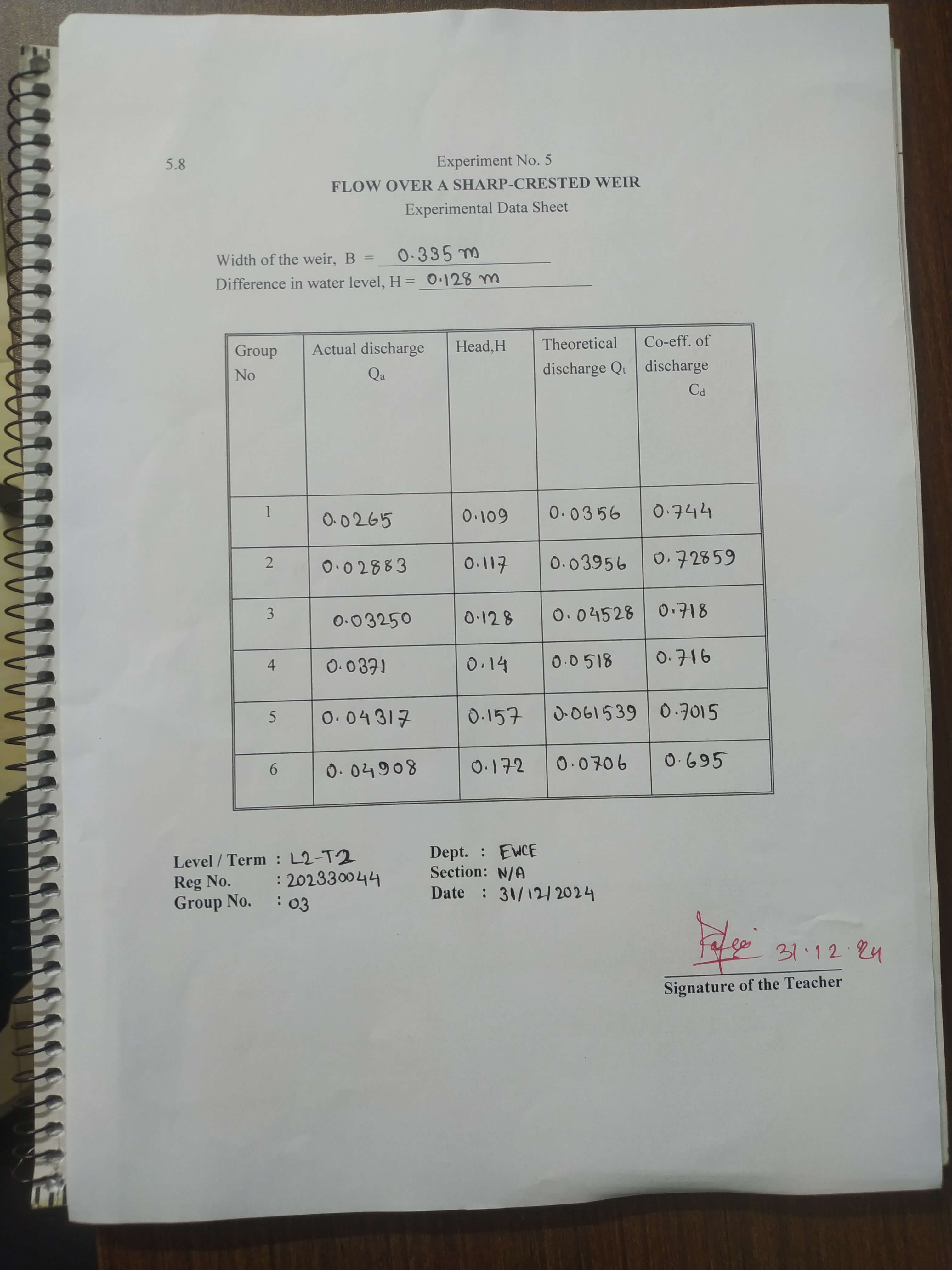
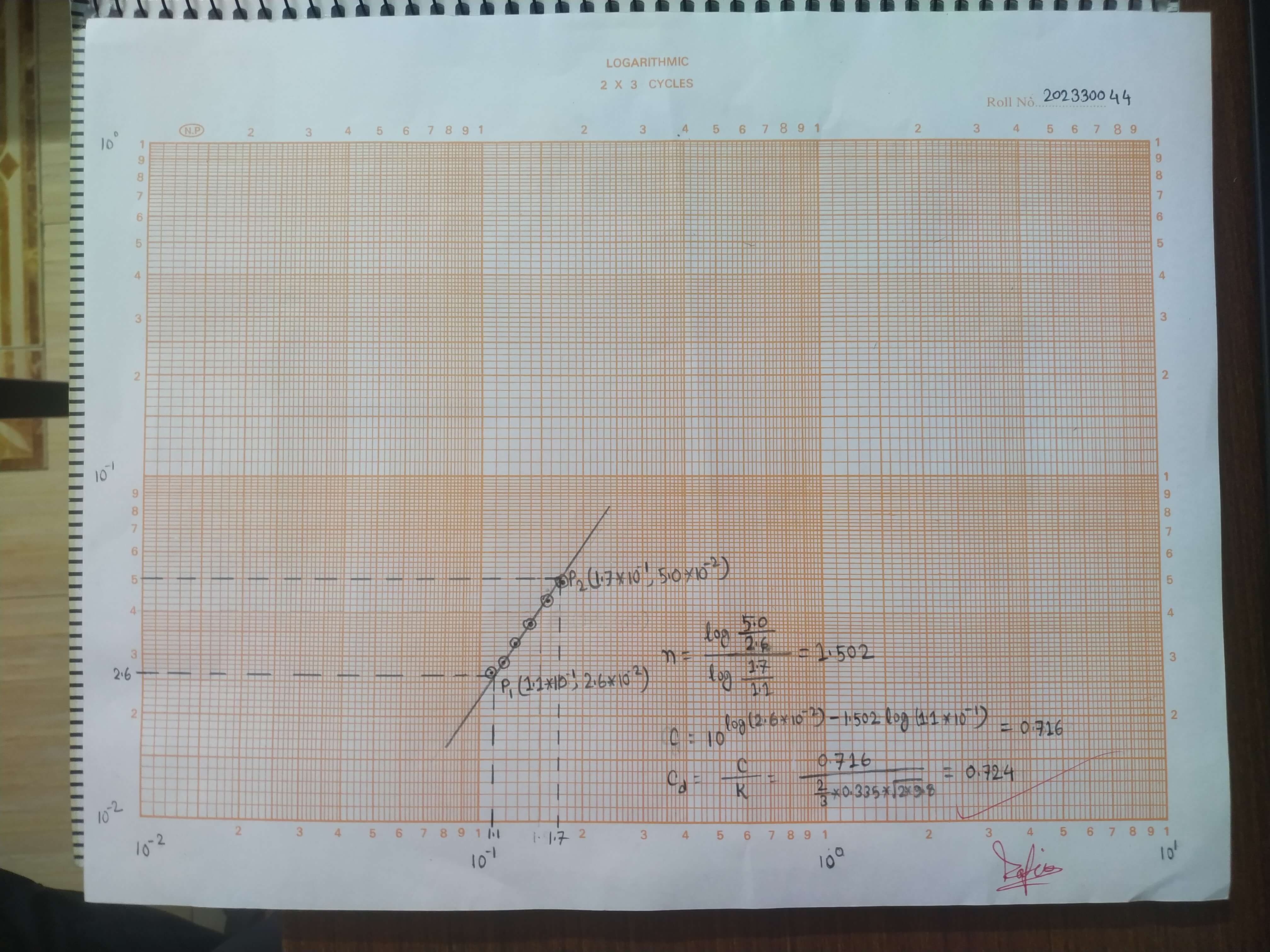
# Calculation
For the two points ($P_1$ and $P_2$) on log-log graph, we get:
1. $H_1 = 1.1\times 10^{-1}$, $Q_1 = 2.6\times 10^{-2}$
2. $H_2 = 1.7\times 10^{-1}$, $Q_2 = 5.0\times 10^{-2}$
The exponent of $H$ can be calculated using the formula,
$$
n = \dfrac{\log{\dfrac{Q_2}{Q_1}}}{\log{\dfrac{H_2}{H_1}}}
$$
Applying the value of $Q_1$, $Q_2$, $H_1$, and $H_2$, we can get,
$$
n = \dfrac{log{\dfrac{5.0\times 10^{-2}}{2.6\times 10^{-2}}}}{\log{\dfrac{1.7\times 10^{-1}}{1.1\times 10^{-1}}}} = 1.502
$$
The calibration parameter $C$ can be calculated using the formula,
$$
C = 10^{\log{Q} - n\log{H}}
$$
Applying the value of $n$, $Q = Q_1$ and $H = H_1$, we can get,
$$
C = 10^{\log{2.6\times 10^{-2}} - 1.502\log{1.1\times 10^{-1}}} = 0.716
$$
Comparing with the calibration equation $Q_a = CH^n$ and $Q_a = KC_dH^n = \dfrac{2}{3}C_d\sqrt{2g}BH^{n}$, the average coefficient of discharge can be calculated using,
$$
C_d = \frac{C}{\dfrac{2}{3}B\sqrt{2g}}
$$
Applying the value of $C$, $B = 0.335\space m$, and $g = 9.8\space ms^{-2}$, we can get average discharge coefficient,
$$
C_d = \frac{0.716}{\dfrac{2}{3}\times 0.335\times \sqrt{2\times 9.8}} = 0.724
$$
# Discussion
In this experiment, the average discharge coefficient ($C_d$) and the exponent of $H$ ($n$) for a selected sharp crested rectangular weir was successfully determined. The values are $0.724$ and $1.502$ respectively. For consecutive use of this weir, the actual discharge can be calculated by measuring only weir head $H$:
$$
Q_a = KC_dH^n = 0.716\times H^{1.502}
$$
## Possible experimental errors
This experiment involves measuring weir head ($H$) and actual discharge ($Q_a$). The later ($Q_a$) is calculated automatically by the machine, however, the former ($H$) is calculated manually. The possible sources of errors are:
1. Inaccurate readings of weir head due to parallax errors or improper settings of the scale.
2. Poorly calibrated or damaged equipment that is measuring actual discharge.
## Ventilation of nappe
As water falls away from the weir, it creates a space with air entrapped beneath the sheet of water. This entrapped air is carried away by the flowing water over time, creating a negative pressure which drags more water resulting in increased discharge. To mitigate this issue, the nappe and weir is ventilated by creating some holes through the channel walls.
## Result and nature of the graph
The experiment yielded values of discharge coefficient, $C_d$, ranging from $0.695$ to $0.744$ with the average (from graph) being $0.724$. It means that, actual discharge is $0.724$ times of theoretical discharge. This is due to the assumptions made when deriving the formula including water is incompressible, flow is uniform and ideal, pressure is atmospheric, etc.
On the other hand, the produced exponent of $H$ ($n$) is $1.502$ which is very close to the theoretical value of $1.5$ indicating that the experiment was well conducted.
The log-log discharge ($Q_a$) vs head ($H$) graph showed a fairly linear relationship between $Q_a$ and $H$. The data points closely follows the straight slope line indicating consistency between $Q_a$ and $H$.
# Practice questions
## 1. Assumptions made in deriving the equation
The assumptions made when deriving the equation $Q_t = \frac{2}{3}B\sqrt{2g}H^{\frac{3}{2}}$ are:
1. The flow is assumed to be uniform.
2. The free surface is assumed to be horizontal as far as the plane of the weir. Realistically, it drops as it approaches the weir.
3. The upstream velocity, effects of viscosity, and surface tension are neglected.
4. The pressure throughout the sheet of liquid is assumed to be atmospheric.
## 2. Pressure distribution over the weir-crest is less than hydrostatic
The pressure distribution over the weir crest is less than hydrostatic due to:
1. As water flows over the sharp crest its velocity increases due to gravity. As per Bernoulli's equation, increased velocity results in decreased pressure.
2. Frictional losses at the crest area causes energy loss resulting in reduced pressure.
## 3. Ventilation below nappe
Ventilating the space below nappe is necessary to:
1. Maintaining pressure distribution. As water flows over the crest, it drags the entrapped air below it, resulting in reduced pressure below the nappe which may cause increased discharge.
2. When the space below is ventilated, atmospheric pressure is maintained ensuring proper flow conditions.
## 4. Effects of lateral contraction
- Lateral contraction reduces the effective width of the flow over the weir. This causes a narrower nappe, which decreases the cross-sectional area available for the flow.
- Decreased cross-sectional area results in increased velocity as per continuity equation.
- Lateral contraction increases energy loss resulting in lower discharge coefficient ($C_d$).
## 5. Mathematical problem
Here,
- Width of the weir, $B = 8\space ft$
- Weir head, $H = 1.20\space ft$
Therefore, discharge,
$$
Q_t = \frac{2}{3}B\sqrt{2g}H^{\dfrac{3}{2}} = \frac{2}{3}\times 8\times \sqrt{2\times 32.17}\times 1.20^{\dfrac{3}{2}} = 56.24\space ft^3/s
$$